Data transformation is a crucial step in the data analysis process, and it is the process of converting raw data into a format that is more suitable for analysis. Two popular tools for data transformation are R-tidyverse and Python-pandas. Both of these tools are widely used by data scientists and analysts, but they have different strengths and weaknesses.
R-tidyverse is a collection of R packages designed for data science, including packages for data manipulation (dplyr, tidyr), data visualization (ggplot2), and data analysis (purrr, lubridate, etc.). Its main strength is its ability to make data manipulation and transformation simple, readable and explicit with its consistent grammar and pipe operator. Additionally, it has a wide range of tools available for data manipulation and cleaning. However, one of its weaknesses is that it can be slower than other alternatives when dealing with very large datasets.
Python-pandas is a powerful library for data manipulation and transformation in Python. It offers a wide range of data structures and data manipulation functions. One of its main strengths is its ability to handle large datasets efficiently. Additionally, it is widely used in the data science community and has a large number of resources available online. On the other hand, one of its weaknesses is that the syntax for data manipulation can be less explicit and more verbose than in R-tidyverse.
The following code example compares the data transformation process using R-tidyverse and Python-pandas
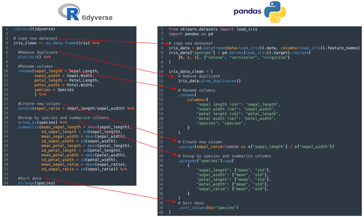
Example in R-tidyverse:
					library(tidyverse)

# copy new datasest
iris_clean <- as.data.frame(iris) %>%

  #Remove duplicate
  distinct() %>%

  #Rename columns
  rename(sepal_length = Sepal.Length,
         sepal_width = Sepal.Width,
         petal_length = Petal.Length,
         petal_width = Petal.Width,
         species = Species
         ) %>%

  #Create new column
  mutate(sepal_ratio = sepal_length/sepal_width) %>%

  #Group by species and summarize columns
  group_by(species) %>%
  summarize(mean_sepal_length = mean(sepal_length),
            sd_sepal_length = sd(sepal_length),
            mean_sepal_width = mean(sepal_width),
            sd_sepal_width = sd(sepal_width),
            mean_petal_length = mean(petal_length),
            sd_petal_length = sd(petal_length),
            mean_petal_width = mean(petal_width),
            sd_petal_width = sd(petal_width),
            mean_sepal_ratio = mean(sepal_ratio),
            sd_sepal_ratio = sd(sepal_ratio)) %>%

  #Sort data
  arrange(species)
Example in Python-pandas
					from sklearn.datasets import load_iris
import pandas as pd

# copy new datasest
iris_data = pd.DataFrame(data=load_iris().data, columns=load_iris().feature_names)
iris_data["species"] = pd.Series(load_iris().target).replace(
    [0, 1, 2], ["setosa", "versicolor", "virginica"]
)

iris_data_clean = (
    # Remove duplicate
    iris_data.drop_duplicates()

    # Rename columns
    .rename(
        columns={
            "sepal length (cm)": "sepal_length",
            "sepal width (cm)": "sepal_width",
            "petal length (cm)": "petal_length",
            "petal width (cm)": "petal_width",
            "species": "species",
        }
    )

    # Create new column
    .assign(sepal_ratio=lambda x: x["sepal_length"] / x["sepal_width"])

    # Group by species and summarize columns
    .groupby("species").agg(
        {
            "sepal_length": ["mean", "std"],
            "sepal_width": ["mean", "std"],
            "petal_length": ["mean", "std"],
            "petal_width": ["mean", "std"],
            "sepal_ratio": ["mean", "std"],
        }
    )
    # Sort data
    .sort_values(by="species")
)